Summary of Models
This page contains high-level documentation about the available models, check the classes doc strings, or the online documentation, for the specific arguments.
The input template maps for many models are available at NERSC on the cmb project space at:
/global/project/projectdirs/cmb/www/so_pysm_models_data
they are also published via web at http://portal.nersc.gov/project/cmb/so_pysm_models_data/.
GaussianSynchrotron
This class implements Gaussian simulations for Galactic synchrotron emission. The inputs are a bunch of parameters defining the properties of the synchrotron power spectra, and of synchrotron Spectral Energy Distribution (SED), the output are the stokes IQU maps simulated as Gaussian random fields of the defined spectra. In particular, synchrotron power spectra \(C_{\ell}\) are assumed to follow a power law as a function of \(\ell\): \(C_{\ell}^{TT/TE/EE/BB}\propto\ell^{\alpha}\). Spectra are defined by:
The slope \(\alpha\) (same for all the spectra)
The amplitude of TT and EE spectra at \(\ell=80\),
The ratio between B and E-modes
Stokes Q and U maps are generated as random realization of the polarization spectra. For the temperature map the situation is slightly different as we want the total intensity map to be positive everywhere. The Stokes I map is generated in the following way:
- if target \(N_{side}<=64\):
The TT power spectrum is \(C_\ell \propto \ell^\alpha\) and \(C_\ell[0]=0\)
A first temperature map T is generated as a gaussian realization of this power spectrum
A new map is obtained by adding to T an offset whose value is taken from a reference map
If T+offset is positive everywhere than this is the output temperature map
Otherwise a cut in the TT power spectrum is applied in the following way: \(C_\ell[1:\ell_{cut}] = C_\ell[\ell_{cut}]\)
A new \(T+offset\) map is generated. The value of \(\ell_{cut}\) is the minimum one for which \(T+offset\) is positive everywhere
- if target \(N_{side}>64\):
a map at \(N_{side}=64\) is generated following the procedure above and then filtered to retain only large angular scales (ell<30)
a map at the target \(N_{side}\) is generated including only small scales (ell>30) with the same seed as the map at point 1.
the two maps are added together
In case the co-added map still has negative pixels a small offset is added to make it positive everywhere
The default parameters are optimized for SO-SAT observations. Meaning that the amplitudes of power spectra are normalized in the 10% sky region observed by the instrument. In particular:
1. The amplitude of TT spectrum is taken from PySM-s0 model at 23GHz. TT_amplitude = 20 \(\mu K^2\) (for \(D_\ell\) at \(\ell=80\))
1. The offset for T map is also taken from PySM-s0 model at 23GHz. Toffset = 72 \(\mu K\)
1. The amplitude of EE spectrum is taken from S-PASS at 2.3GHz extrapolated at 23GHz with a power-law with \(\beta_s=-3.1\) EE_amplitude = 4.3 math:mu K^2 (for \(D_\ell\) at \(\ell=80\))
1. ratio between B and E modes from Krachmalnicoff et al. 2018, B_to_E = 0.5
1. spectral tilt from Krachmalnicoff et al 2018, alpha = -1
1. spectral index from Planck IX 2018, beta = -3.1
1. Default value for curvature is zero
GaussianDust
This class implements Gaussian simulations for Galactic thermal dust emission. The inputs are a bunch of parameters defining the properties of dust power spectra, and of dust Spectral Energy Distribution (SED), the output are the stokes IQU maps simulated as Gaussian random fields of the defined spectra. In particular, dust power spectra \(C_{\ell}\) are assumed to follow a power law as a function of \(\ell\): \(C_{\ell}^{TT/TE/EE/BB}\propto\ell^{\alpha}\). Spectra are defined by:
The slope \(\alpha\) (same for all the spectra)
The amplitude of TT and EE spectra at \(\ell=80\),
The ratio between B and E-modes
The degree of correlation between T and E.
Stokes Q and U maps are generated as random realization of the polarization spectra. For the temperature map the situation is slightly different as we want the total intensity map to be positive everywhere. The Stokes I map is generated in the following way:
- if target \(N_{side}<=64\):
The TT power spectrum is \(C_\ell \propto \ell^\alpha\) and \(C_\ell[0]=0\)
A first temperature map T is generated as a gaussian realization of this power spectrum
A new map is obtained by adding to T an offset whose value is taken from a reference map
If T+offset is positive everywhere than this is the output temperature map
Otherwise a cut in the TT power spectrum is applied in the following way: \(C_\ell[1:\ell_{cut}] = C_\ell[\ell_{cut}]\)
A new \(T+offset\) map is generated. The value of \(\ell_{cut}\) is the minimum one for which \(T+offset\) is positive everywhere.
- if target \(N_{side}>64\):
a map at \(N_{side}=64\) is generated following the procedure above and then filtered to retain only large angular scales (ell<30)
a map at the target \(N_{side}\) is generated including only small scales (ell>30) with the same seed as the map at point 1.
the two maps are added together
In case the co-added map still has negative pixels a small offset is added to make it positive everywhere
Typical values for \(\ell_{cut}\) are between \(\ell=4\) and \(\ell=9\), depending on realization (and also on the \(N_{side}\) of the output map). This implementation removes some power at the very large scales.
The default parameters are optimized for SO-SAT observations. Meaning that the amplitudes of power spectra are normalized in the 10% sky region observed by the instrument. In particular:
The amplitude of TT spectrum is taken from PySM-d0 model at 353GHz. TT_amplitude = 350 \(\mu K^2\) (for \(D_\ell\) at \(\ell=80\))
The offset for T map is also taken from PySM-d0 model at 353GHz. Toffset = 18 \(\mu K\)
The amplitude of EE spectrum is taken from Planck map at 353GHz, EE_amplitude = 100 math:
mu K^2(for \(D_\ell\) at \(\ell=80\))ratio between B and E modes from Planck IX 2018, B_to_E = 0.5
spectral tilt from Planck IX 2018, alpha = -0.42
spectral index and temperature from Planck IX 2018, beta = 1.53, T=19.6 K
COLines
COLines is not a standard PySM component because PySM does not allow to distinguish between a case where a component is evaluated for the purpose of integrating over the bandpass or evaluated for separate channels.
Therefore this class should be instantiated choosing the desired line and summed to the output of PySM.
For example:
from so_pysm_models import COLines
co = COLines(nside=16, output_units="uK_CMB", line="10")
pysm_map += bandpass_weight * hp.smoothing(co.signal(), fwhm=fwhm)
Where bandpass_weight is the scalar transmission at the line frequency (which is available at co.line_frequency), i.e. if the bandpass is a top-hat between 110 and 120 GHz, the “10” line emission should be multiplied by 0.1.
This class implements simulations for Galactic CO emission involving the first 3 CO rotational lines, i.e. \(J=1-0,2-1,3-2\) whose center frequency is respectively at \(\nu_0 = 115.3, 230.5,345.8\) GHz. The CO emission map templates are the CO Planck maps obtained with MILCA component separation algorithm (See Planck paper). The CO maps have been released at the nominal resolution (10 and 5 arcminutes). However, to reduce noise contamination from template maps (especially at intermediate and high Galactic latitudes), we convolved them with a 1 deg gaussian beam.
The Stokes I map is computed from the template one as it follows:
if target \(N_{side}\) <= 512:
The template map at a
nside=512is downgraded at the target \(N_{side}\)
if target \(N_{side}\) > 512 :
The template map at a
nside=2048is downgraded(eventually upgraded) at the target \(N_{side}\)
Q and U maps can be computed from the template CO emission map, \(I_{CO}\), assuming a constant fractional polarization, as:
with \(g_d\) and \(\psi\) being respectively the depolarization and polarization angle maps estimated from a dust map as :
Most of the CO emission is expected to be confined in the Galactic midplane. However, there are still regions at high Galactic latitudes where the CO emission has been purely assessed (by current surveys) and where the Planck signal-to-noise was not enough to detect any emission.
The PySM user can include the eventuality of molecular emission (both unpolarized and polarized) at High Gal. Latitudes by co-adding to the emission maps one realization of CO emission simulated with MCMole3D together with the Planck CO map. The polarization is simulated similarly as above.
The MCMole3D input parameters are are obtained from best fit with the Planck CO 1-0 map (see Puglisi et al. 2017 and the documentation). If include_high_galactic_latitude_clouds=True, a mock CO cloud map is simulated with MCMole3D, encoding high Galactic latitudes clouds at latitudes above and below than 20 degrees. The mock emission map is then co-added to the Planck CO emission map. The polarization is simulated similarly as above.
The installation of mcmole3d is not required, HGL clouds can be input to the CO emission by setting run_mcmole3d=False (which is the default). However, if one wants to run several mock CO realizations observing high Galactic latitude patches we encourage to run mcmole3d by changing random_seed in the CO class constructor. The parameter theta_high_galactic_latitude_deg set the latitude above which CO emission from high Galactic latitudes can be included and it has an impact only when run_mcmole3d=True.
The default parameters are set to include CO 1-0 emission and polarization (with 0.1% constant polarization fraction), in particular:
polarization_fraction= 0.001, on average is the expected level on 10% regions of the sky. However, polarization from CO emission have been detected at larger fluxes in Orion and Taurus complexes (Greaves et al.1999 )
theta_high_galactic_latitude_deg = 20, includes CO emission at \(|b|>\theta_{hgl}\) from one realization of mcmole3d maps. Be aware that the larger \(theta_{hgl}\), the farther is the Galactic plane and the more unlikely is to find high Galactic latitude clouds.
PrecomputedAlms
This class generates a PySM component based on a set of pre-computed \(a_{\ell,m}\) coefficients stored in a folder
in FITS format.
This is mostly targeted at simulations of the Cosmic Microwave Background, the input \(a_{\ell,m}\) can be in
K_{RJ} or K_{CMB} as defined in the constructor, the unit conversion is performed assuming the CMB black body spectrum.
The output unit is specified in the signal method, default is mu K_{RJ}, as expected by PySM.
In case the input is in K_{RJ}, it is necessary also to specify input_reference_frequency_GHz.
The transformation between Spherical Harmonics and pixel domain can be performed either during initialization or in the
signal method based on precompute_output_map.
See the documentation about mapsims about specific simulated datasets.
InterpolatingComponent
Moved to PySM 3, FIXME port this documentation over
Adds a custom emission to the sky simulated by PySM defined as a set of template maps at pre-defined frequencies to be interpolated at the frequencies requested through PySM.
Inputs
A folder of maps named with their frequency in GHz with the flux in any unit supported
by PySM (e.g. Jysr, MJsr, uK_RJ, K_CMB). They don’t need to be equally spaced
For example:
ls `cib_precomputed_maps/`
0010.0.fits 0015.0.fits 0018.0.fits
Usage
Instantiate InterpolatingComponent and point it to the folder, define the unit and the target \(N_{side}\) (same used by PySM).
It supports all interpolation_kind of scipy.interpolate.interp1d(), e.g. “nearest”, “linear”, “quadratic”, “cubic”:
cib = InterpolatingComponent(path="cib_precomputed_maps", input_units="MJysr", target_nside=nside, interpolation_kind="linear",
                         has_polarization=False, verbose=True)
WebSky
The Websky suite of simulated extragalactic component maps, determined from large scale structure light cone realizations and based on Lagrangian perturbation theory, Peak Patch Lagrangian halo finding, and modeling of SZ and CIB effects, can be read into PySM as precomputed external fits files using InterpolatingComponent. More information on the Peak Patch halo finding method can be found in Stein, Alvarez, and Bond (2018), and selected maps and halo catalogs are available from the Websky website. Some additional Websky-specific information and tools are available at the SO Websky model repository.
The cosmological parameters used for the websky simulations are available at on the websky website.
Specific maps generated for so_pysm_models are described below and located on NERSC at /project/projectdirs/sobs/v4_sims/mbs/websky/0.3.
Cosmic Infrared Background
The Planck (2013) CIB halo model is used, along with a halo occupation distribution. More details can be found here.
The current version of the maps are of intensity in units of \(MJy/Sr\) with filename convention cib_nu[FREQ].fits e.g. cib_nu0027.fits is the map of CIB intensity at 27 GHz and will be used by InterpolatingComponent() at that frequency, and can be found on NERSC at /project/projectdirs/sobs/v4_sims/mbs/websky/0.3. There are 18 fits files at \(N_{side}=4096\) at frequencies [27, 39, 93, 145, 225, 280] +/- 1 GHz, in addition to those corresponding to the Planck HFI channel centers, [100, 143, 217, 353, 545, 857] GHz, for a total of 24 files. These intensities were selected because in order to be able to interpolate accurately at the 6 frequencies of interest with as few maps as possible. More frequencies will be made available after a full set of map based simulations at SO bands that include correlated lensing, CIB, and SZ effects has been generated.
Thermal SZ Effect
Provided is a map of the Compton-y parameter and is based on Battaglia et al. (2012) pressure profiles, and can be found at /project/projectdirs/sobs/v4_sims/mbs/websky/0.3/tsz.fits.
Kinetic SZ Effect
Provided is a map of the temperature fluctuation due to line of sight peculiar velocities of electrons along the line of sight. Electrons are assumed to follow a Navarro Frenk and White (NFW) profile interior to halos and second order Lagrangian Perturbation Theory (LPT) outside. The ksz map can be found at /project/projectdirs/sobs/v4_sims/mbs/websky/0.3/ksz.fits.
Lensing Convergence
A lensing convergence map is generated from the simulated matter distribution along the line of sight, assumed to follow an NFW profile interior to halos and second order LPT outside.
Primary and lensed CMB The convergence map is used to lens a Gaussian realization of the unlensed primary CMB, which is then read into PySM as the primary lensed CMB through the PrecomputedAlms class. The primary CMB is obtained from parameters that match the Websky simulation, namely A_s = 2.022e-9, tau = 0.055, and all other parameters set to the websky values above, see the code, values not explicitely set are equal to the CAMB default, for example \(N_{eff}=3.046\) . The CAR maps (where the lens remapping is done) have 1 arcminute resolution.
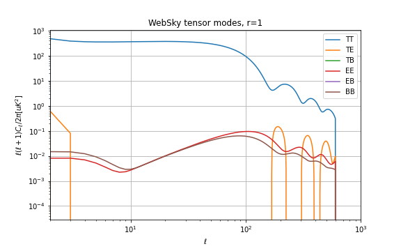
The theoretical power spectra for the unlensed and lensed CMB are available here https://github.com/ajvanengelen/webskylensing/tree/master/data. Each is a numpy array of shape (3, 3, N_l), giving the theory power spectrum C_l’s in the order ((TT, TE, TB), (ET, EE, EB), (BT, BE, BB)) in units of uK_CMB^2. They are obtained from the get_cmb_powerspecta.websky_cmb_spectra routine in that repository, which serves as a wrapper to CAMB.
The WebSkyCMBTensor provides the \(BB\) spectrum for the Websky cosmology from a model with \(r = 1\) (which of course needs to be scaled to whatever actual \(r\) value we want to use). This component is not lensed.
The tensor spectral index (\(n_t\)) in CAMB was set to 0.
The \(C_\ell\) from CAMB has power only up to \(\ell = 600\), however, given that the primordial BB signal is suppressed on scales smaller than the horizon scale at decoupling this should not matter in practice, for more details see this Github issue